Pumpkins
From a blog-post by Julia Silge Julia Silge’s blog of Tidymodels Giant Pumpkins
Let’s train a model for giant pumpkins, predicting a giant pumpkin weight from other characteristics
Explore Data
library(tidyverse)

pumpkins_raw <- readr::read_csv("https://raw.githubusercontent.com/rfordatascience/tidytuesday/master/data/2021/2021-10-19/pumpkins.csv")
## Rows: 28065 Columns: 14## -- Column specification --------------------------------------------------------
## Delimiter: ","
## chr (14): id, place, weight_lbs, grower_name, city, state_prov, country, gpc...##
## i Use `spec()` to retrieve the full column specification for this data.
## i Specify the column types or set `show_col_types = FALSE` to quiet this message.pumpkins <-
pumpkins_raw %>%
separate(id, into = c("year", "type")) %>%
mutate(across(c(year, weight_lbs, ott, place), parse_number)) %>%
filter(type == "P") %>%
select(weight_lbs, year, place, ott, gpc_site, country)## Warning: 2327 parsing failures.
## row col expected actual
## 13 -- a number EXH
## 36 -- a number EXH
## 58 -- a number EXH
## 60 -- a number EXH
## 61 -- a number EXH
## ... ... ........ ......
## See problems(...) for more details.pumpkins## # A tibble: 15,965 x 6
## weight_lbs year place ott gpc_site country
## <dbl> <dbl> <dbl> <dbl> <chr> <chr>
## 1 2032 2013 1 475 Uesugi Farms Weigh-off United Sta~
## 2 1985 2013 2 453 Safeway World Championship Pumpkin ~ United Sta~
## 3 1894 2013 3 445 Safeway World Championship Pumpkin ~ United Sta~
## 4 1874. 2013 4 436 Elk Grove Giant Pumpkin Festival United Sta~
## 5 1813 2013 5 430 The Great Howard Dill Giant Pumpkin~ Canada
## 6 1791 2013 6 431 Elk Grove Giant Pumpkin Festival United Sta~
## 7 1784 2013 7 445 Uesugi Farms Weigh-off United Sta~
## 8 1784. 2013 8 434 Stillwater Harvestfest United Sta~
## 9 1780. 2013 9 422 Stillwater Harvestfest United Sta~
## 10 1766. 2013 10 425 Durham Fair Weigh-Off United Sta~
## # ... with 15,955 more rowsThe main relationship here is between the volume/size of the pumpkin (measured via “over-the-top inches”) and weight.
pumpkins %>%
  filter(ott > 20, ott < 1e3) %>%
  ggplot(aes(ott, weight_lbs, color = place)) +
  geom_point(alpha = 0.2, size = 1.1) +
  labs(x = "over-the-top inches", y = "weight (lbs)") +
  scale_color_viridis_c()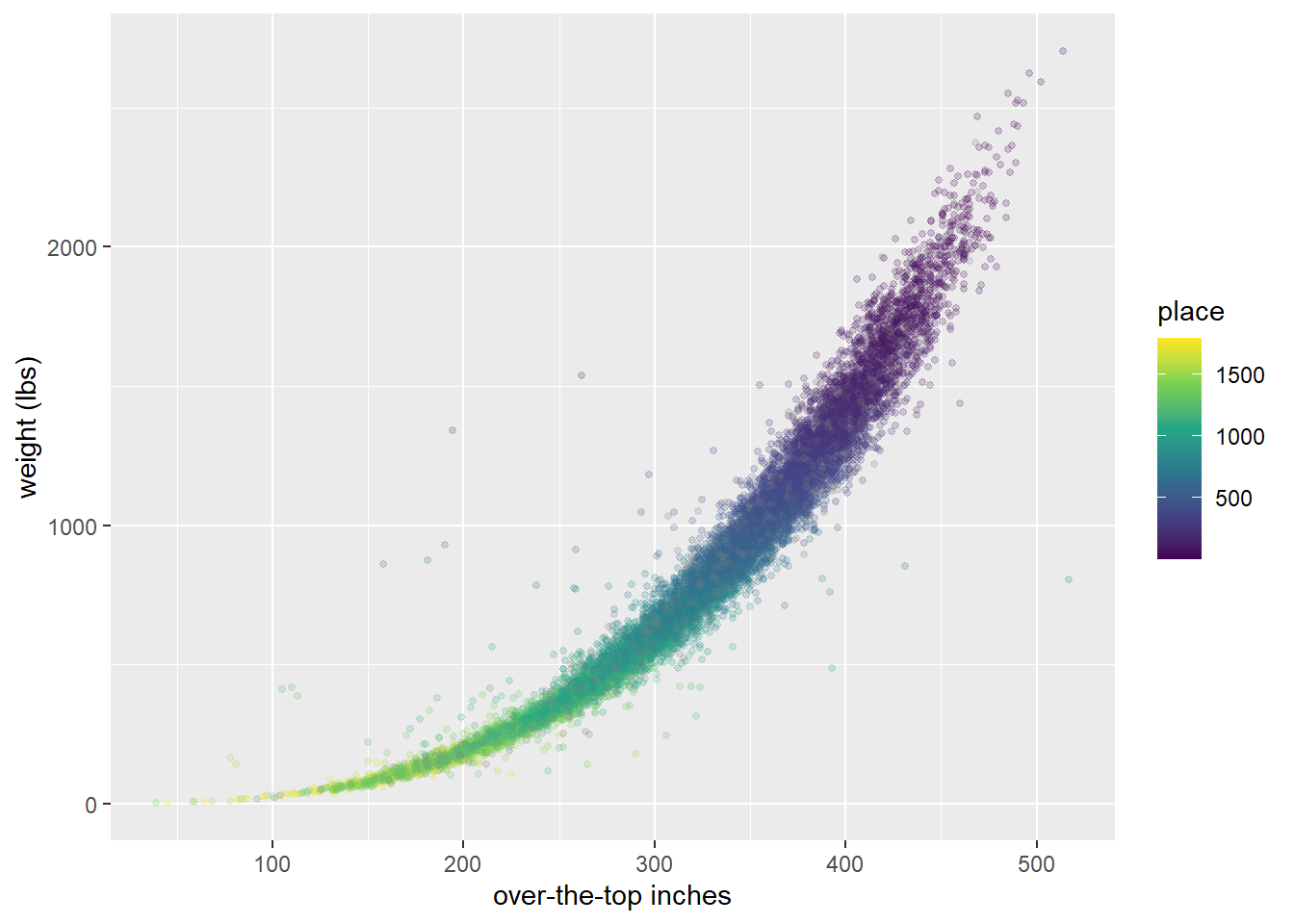
Big, heavy pumpkins placed closer to winning at the competitions, naturally!
Has there been any shift in this relationship over time?
pumpkins %>%
  filter(ott > 20, ott < 1e3) %>%
  ggplot(aes(ott, weight_lbs)) +
  geom_point(alpha = 0.2, size = 1.1, color = "gray60") +
  geom_smooth(aes(color = factor(year)),
    method = lm, formula = y ~ splines::bs(x, 3),
    se = FALSE, size = 1.5, alpha = 0.6
  ) +
  labs(x = "over-the-top inches", y = "weight (lbs)", color = NULL) +
  scale_color_viridis_d()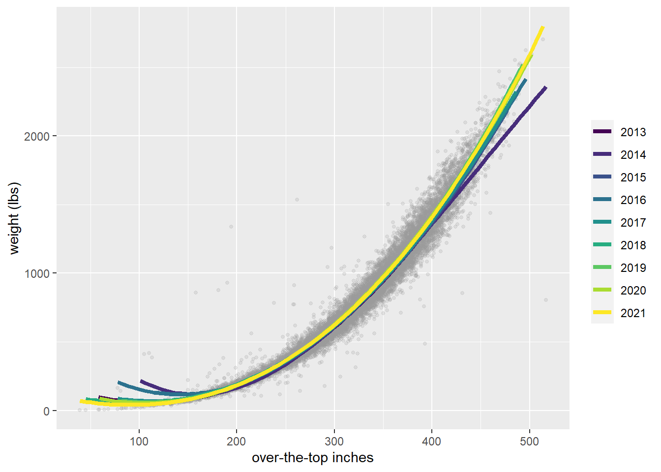
Hard to say, I think.
Which countries produced more or less massive pumpkins?
pumpkins %>%
  mutate(
    country = fct_lump(country, n = 10),
    country = fct_reorder(country, weight_lbs)
  ) %>%
  ggplot(aes(country, weight_lbs, color = country)) +
  geom_boxplot(outlier.colour = NA) +
  geom_jitter(alpha = 0.1, width = 0.15) +
  labs(x = NULL, y = "weight (lbs)") +
  theme(legend.position = "none")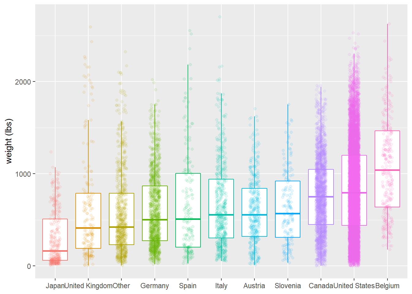
Build and fit a workflow set
library(tidymodels)## Registered S3 method overwritten by 'tune':
## method from
## required_pkgs.model_spec parsnip## -- Attaching packages -------------------------------------- tidymodels 0.1.4 --## v broom 0.7.10 v rsample 0.1.1
## v dials 0.0.10 v tune 0.1.6
## v infer 1.0.0 v workflows 0.2.4
## v modeldata 0.1.1 v workflowsets 0.1.0
## v parsnip 0.1.7 v yardstick 0.0.9
## v recipes 0.1.17## Warning: package 'rsample' was built under R version 4.1.2## Warning: package 'yardstick' was built under R version 4.1.2## -- Conflicts ----------------------------------------- tidymodels_conflicts() --
## x scales::discard() masks purrr::discard()
## x dplyr::filter() masks stats::filter()
## x recipes::fixed() masks stringr::fixed()
## x dplyr::lag() masks stats::lag()
## x yardstick::spec() masks readr::spec()
## x recipes::step() masks stats::step()
## * Dig deeper into tidy modeling with R at https://www.tmwr.orgset.seed(123)
pumpkin_split <- pumpkins %>%
filter(ott > 20, ott < 1e3) %>%
initial_split(strata = weight_lbs)
pumpkin_train <- training(pumpkin_split)
pumpkin_test <- testing(pumpkin_split)
set.seed(234)
pumpkin_folds <- vfold_cv(pumpkin_train, strata = weight_lbs)
pumpkin_folds## # 10-fold cross-validation using stratification
## # A tibble: 10 x 2
## splits id
## <list> <chr>
## 1 <split [8954/996]> Fold01
## 2 <split [8954/996]> Fold02
## 3 <split [8954/996]> Fold03
## 4 <split [8954/996]> Fold04
## 5 <split [8954/996]> Fold05
## 6 <split [8954/996]> Fold06
## 7 <split [8955/995]> Fold07
## 8 <split [8956/994]> Fold08
## 9 <split [8957/993]> Fold09
## 10 <split [8958/992]> Fold10Next, let’s create three data preprocessing recipes: one that only pools infrequently used factors levels, one that also creates indicator variables, and finally one that also creates spline terms for over-the-top inches.
base_rec <-
  recipe(weight_lbs ~ ott + year + country + gpc_site,
    data = pumpkin_train) %>%
  step_other(country, gpc_site, threshold = 0.02)

ind_rec <-
  base_rec %>%
  step_dummy(all_nominal_predictors())

spline_rec <-
  ind_rec %>%
  step_bs(ott)
Then, let’s create three model specifications: a random forest model, a MARS model, and a linear model.
rf_spec <-
  rand_forest(trees = 1e3) %>%
  set_mode("regression") %>%
  set_engine("ranger")

mars_spec <-
  mars() %>%
  set_mode("regression") %>%
  set_engine("earth")

lm_spec <- linear_reg()
Now it’s time to put the preprocessing and models together in a workflow_set().
pumpkin_set <-
  workflow_set(
    list(base_rec, ind_rec, spline_rec),
    list(rf_spec, mars_spec, lm_spec),
    cross = FALSE)
pumpkin_set
## # A workflow set/tibble: 3 x 4
## wflow_id info option result
## <chr> <list> <list> <list>
## 1 recipe_1_rand_forest <tibble [1 x 4]> <opts[0]> <list [0]>
## 2 recipe_2_mars <tibble [1 x 4]> <opts[0]> <list [0]>
## 3 recipe_3_linear_reg <tibble [1 x 4]> <opts[0]> <list [0]>We use cross = FALSE because we don’t want every combination of these components, only three options to try. Let’s fit these possible candidates to our resamples to see which one performs best.
library(doParallel)## Warning: package 'doParallel' was built under R version 4.1.2## Loading required package: foreach##
## Attaching package: 'foreach'## The following objects are masked from 'package:purrr':
##
## accumulate, when## Loading required package: iterators## Loading required package: parallellibrary(ranger)## Warning: package 'ranger' was built under R version 4.1.2library(earth)## Warning: package 'earth' was built under R version 4.1.2## Loading required package: Formula## Loading required package: plotmo## Warning: package 'plotmo' was built under R version 4.1.2## Loading required package: plotrix##
## Attaching package: 'plotrix'## The following object is masked from 'package:scales':
##
## rescale## Loading required package: TeachingDemos## Warning: package 'TeachingDemos' was built under R version 4.1.2registerDoParallel()
set.seed(2021)
pumpkin_rs <-
workflow_map(
pumpkin_set,
"fit_resamples",
resamples = pumpkin_folds
)
pumpkin_rs## # A workflow set/tibble: 3 x 4
## wflow_id info option result
## <chr> <list> <list> <list>
## 1 recipe_1_rand_forest <tibble [1 x 4]> <opts[1]> <rsmp[+]>
## 2 recipe_2_mars <tibble [1 x 4]> <opts[1]> <rsmp[+]>
## 3 recipe_3_linear_reg <tibble [1 x 4]> <opts[1]> <rsmp[+]>Evaluate workflow set
How did our three candidates do?
autoplot(pumpkin_rs)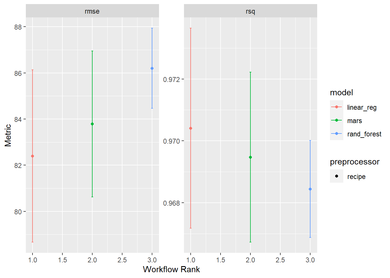
There is not much difference between the three options, and if anything, our linear model with spline feature engineering maybe did better. This is nice because it’s a simpler model!
collect_metrics(pumpkin_rs)## # A tibble: 6 x 9
## wflow_id .config preproc model .metric .estimator mean n std_err
## <chr> <chr> <chr> <chr> <chr> <chr> <dbl> <int> <dbl>
## 1 recipe_1_r~ Preprocess~ recipe rand_~ rmse standard 86.2 10 1.05e+0
## 2 recipe_1_r~ Preprocess~ recipe rand_~ rsq standard 0.968 10 9.53e-4
## 3 recipe_2_m~ Preprocess~ recipe mars rmse standard 83.8 10 1.92e+0
## 4 recipe_2_m~ Preprocess~ recipe mars rsq standard 0.969 10 1.67e-3
## 5 recipe_3_l~ Preprocess~ recipe linea~ rmse standard 82.4 10 2.27e+0
## 6 recipe_3_l~ Preprocess~ recipe linea~ rsq standard 0.970 10 1.97e-3We can extract the workflow we want to use and fit it to our training data.
final_fit <-
  extract_workflow(pumpkin_rs, "recipe_3_linear_reg") %>%
  fit(pumpkin_train)
tidy(final_fit)
## # A tibble: 15 x 5
## term estimate std.error statistic p.value
## <chr> <dbl> <dbl> <dbl> <dbl>
## 1 (Intercept) -9731. 675. -14.4 1.30e- 46
## 2 year 4.89 0.334 14.6 5.03e- 48
## 3 country_Canada 9.29 6.12 1.52 1.29e- 1
## 4 country_Germany -11.5 6.68 -1.71 8.64e- 2
## 5 country_Italy 8.12 7.02 1.16 2.47e- 1
## 6 country_United.States 11.9 5.66 2.11 3.53e- 2
## 7 country_other -10.7 6.33 -1.69 9.13e- 2
## 8 gpc_site_Elk.Grove.Giant.Pumpkin.Fest~ -7.81 7.70 -1.01 3.10e- 1
## 9 gpc_site_Ohio.Valley.Giant.Pumpkin.Gr~ 21.1 7.80 2.70 6.89e- 3
## 10 gpc_site_Stillwater.Harvestfest 11.6 7.87 1.48 1.40e- 1
## 11 gpc_site_Wiegemeisterschaft.Berlin.Br~ 1.51 8.07 0.187 8.51e- 1
## 12 gpc_site_other 1.41 5.60 0.251 8.02e- 1
## 13 ott_bs_1 -345. 36.3 -9.50 2.49e- 21
## 14 ott_bs_2 450. 11.9 37.9 2.75e-293
## 15 ott_bs_3 2585. 25.6 101. 0We can use an object like this to predict, such as on the test data like predict(final_fit, pumpkin_test), or we can examine the model parameters.
tidy(final_fit) %>%
  arrange(-abs(estimate))
## # A tibble: 15 x 5
## term estimate std.error statistic p.value
## <chr> <dbl> <dbl> <dbl> <dbl>
## 1 (Intercept) -9731. 675. -14.4 1.30e- 46
## 2 ott_bs_3 2585. 25.6 101. 0
## 3 ott_bs_2 450. 11.9 37.9 2.75e-293
## 4 ott_bs_1 -345. 36.3 -9.50 2.49e- 21
## 5 gpc_site_Ohio.Valley.Giant.Pumpkin.Gr~ 21.1 7.80 2.70 6.89e- 3
## 6 country_United.States 11.9 5.66 2.11 3.53e- 2
## 7 gpc_site_Stillwater.Harvestfest 11.6 7.87 1.48 1.40e- 1
## 8 country_Germany -11.5 6.68 -1.71 8.64e- 2
## 9 country_other -10.7 6.33 -1.69 9.13e- 2
## 10 country_Canada 9.29 6.12 1.52 1.29e- 1
## 11 country_Italy 8.12 7.02 1.16 2.47e- 1
## 12 gpc_site_Elk.Grove.Giant.Pumpkin.Fest~ -7.81 7.70 -1.01 3.10e- 1
## 13 year 4.89 0.334 14.6 5.03e- 48
## 14 gpc_site_Wiegemeisterschaft.Berlin.Br~ 1.51 8.07 0.187 8.51e- 1
## 15 gpc_site_other 1.41 5.60 0.251 8.02e- 1The spline terms are by far the most important, but we do see evidence of certain sites and countries being predictive of weight (either up or down) as well as a small trend of heavier pumpkins with year.
Don’t forget to take the tidymodels survey for 2022 priorities!
Edward Hillenaar
Writer - Data Scientist - Philosopher
My research interests include psychology, philosophy and data science of the origin and nature of human consciousness.